The main principle behind free energy is that the fundamental psychological drive of organisms is the reduction of uncertainty.

The whole point of variational bayesian methods is that when we want to do a conditional, $p(z | x)$ aka Bayes rule, is intractable because we do not know the normalization constant aka the model evidence $p(x)$.

So we can write out Bayes, solve for evidence, take a log, integrate over the marginalized variable, multiply by approximate posterior, then rewrite in the form with KL divergence plus free energy, solve for that KL divergence, and then maximize free energy which must also implicitly minimize the KL to the posterior at the same time.

This helps us with approximating the posterior predictive distribution,

$$\int p(y^* | x^*, X, Y) = \int p(y^* | x^*, W) \underbrace{p(W | X, Y)}_{\text{posterior}} dW$$

and Active Inference's unified perception and action.

Usmu blog's (link) states it well: "For no matter how the brain arrives at its posterior probability Q, approximating the Bayesian ideal means getting close to the Bayesian posterior P', and getting close the P' means minimizing free energy". Minimizing Friston free energy is equivalent to maximizing the ELBO since ELBO = -F.

As Jim Hopkin notes in the blog, the notion of variational free energy was introduced by Nobel Prize winner, Geoffrey Hinton. Friston's initial inspiration was 'Helmholtz Machine' by Dayan et al 1995. Sungchul Ji also notes that Friston's free energy has nothing to do with Gibbs free energy in thermodynamics, and that Shannon . This was a mass cause of confusion resulted in a rebranding of the Free Energy Principle as Active Inference.

---

JARED TUMIEL Notes

link: https://jaredtumiel.github.io/blog/2020/08/08/free-energy1.html

he uses notation where z=T, x=S

prior: $p(z)$

data: $p(x)$

posterior: intractable

$$p(z|x) = \frac{p(x|z)p(z)}{p(x)}$$ $$= \frac{p(x|z)p(z)}{\int p(x|z)p(x) dz}$$

G-density: Generative Model

$$= p(z,x)$$

R-density: Recognition, aka the approximate posterior or the current best guess of causes of input

$$= q(z)$$

KL-Divergence:

$$D_{KL}(q(z) || p(z|x)) = \int q(z) \log \frac{q(z)}{p(z|x)} dz$$ $$= \int q(z) [\log q(z) - \log p(z|x)] dz$$

Deriving F

$$p(z|x) = \frac{p(x|z)p(z)}{p(x)}$$ $$p(z|x) = \frac{p(z,x)}{p(x)}$$ $$\ln p(z|x) = \ln \frac{p(z,x)}{p(x)}$$ $$\ln p(z|x) = \ln p(z,x) - \ln p(x)$$ $$\text{Plugging into KL Divergence formula:}$$ $$D_{KL}(q(z)||p(z|x)) = \int q(z) [\ln q(z) - \ln p(z,x) + \ln p(x)] dz$$ $$= \int q(z) [\ln \frac{\overbrace{q(z)}^{\text{approximate posterior}}}{\underbrace{p(z,x)}_{\text{world model}}} + \underbrace{\ln p(x)}_{\text{surprisal}}] dz$$ $$= \int q(z) \ln \frac{q(z)}{p(z,x)} dz + \int q(z) \ln p(x) dz$$ $$= \int q(z) \ln \frac{q(z)}{p(z,x)} dz + \ln p(x) \int q(z) dz$$ $$= \int q(z) \ln \frac{q(z)}{p(z,x)} dz + \ln p(x)$$ $$\text{Therefore}$$ $$D_{KL}(q(z)||p(z,x)) = \underbrace{\int q(z) \ln \frac{q(z)}{p(z,x)} dz}_{\text{F}} + \ln p(x)$$ $$= F + \ln p(x)$$ $$= F - (- \ln p(x))$$

Free Energy:

$$= D_{KL} (q(z) || p(z,x))$$ $$= \int q(z) \frac{q(z)}{p(z,x)} dz$$

Free Energy is an upper bound on surprisal: Minimizing this approximates the true posterior p(z|x)

$$D_{KL}(q(z)||p(z|x)) \ge 0$$ $$F + \ln p(x) \ge 0$$ $$F \ge -\ln p(x)$$ $$\text{so therefore we want to minimize F}$$

Hemoltz Free Energy

$$\text{if q(z) == p(z)}$$ $$\int q(z) \ln q(z) dz - \int q(z) p(x,z) dz$$ $$= \mathbb{E}_{q(z)}[\ln q(z)] - \mathbb{E}_{q(z)}[\ln p(x,z)]$$ $$= \underbrace{H(z)}_{\text{entropy}} - \underbrace{E(z,x)}_{\text{energy}}$$ $$= \text{(negative?) Helmholtz Free Energy}$$ $$= \underbrace{U}_{\text{internal energy}}-\underbrace{T}_{\text{temperature}} \cdot \overbrace{x}^{\text{entropy}}$$

---

KAIU Notes

link: https://web.archive.org/web/20210228154305/https://kaiu.me/2017/06/23/deep-active-inference-for-artificial-general-intelligence/

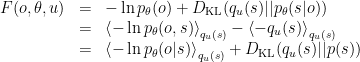
Equivalent forms of the free energy functional:

#1. Agent tied to rock

$$F = D_{KL}(q(z)||p(z,x)) - \ln p(x)$$

#2. Physics Formula

$$F = \mathbb{E}_{q(z)}[\ln q(z)] - \mathbb{E}_{q(z)}[\ln p(x,z)]$$ $$= \mathbb{E}_{q(z)}[- \ln p(x,z)] - \mathbb{E}_{q(z)}[- \ln q(z)]$$

#3. Agent able to take actions

$$F = D_{KL}(q(z)||p(x)) - \mathbb{E}_{q(z)}[\ln p(z|x)]$$

---

Active Inference Book Formulas:

observation y -> x

latent/state x -> z

In reality we work with the negative F

$$$$

\begin{aligned} F[Q,x] &= \underbrace{-\mathbb{E}{q(z)}[\ln p(x,z)]}{\text{Energy}} - \underbrace{H[q(z)]}{\text{Entropy}} \tag{1, k2}\ &= \underbrace{D{KL}(q(z),|,p(z))}{\text{Complexity}} - \underbrace{\mathbb{E}{q(z)}[\ln p(x | z)]}{\text{Accuracy}} \tag{2, k3}\ &= \underbrace{D{KL}(q(z),|,p(z | x))}{\text{Divergence}} - \underbrace{\ln p(x)}{\text{Evidence}} \tag{3, k1} \end{aligned}

$$$$

---

ELBO

aka variational lower bound. minimize variational free energy, maximize variation lower bound

$$$$

\begin{aligned} \text{ELBO} &= -F[Q,x] \ &= -\text{(variational free energy)} \end{aligned}

$$$$

From Introduction to VAE

$Q(z) \leftrightarrow q_{\phi}(z|x)$

$P(z|x) \leftrightarrow p_{\theta}(z|x)$

$$$$

\begin{aligned} \mathcal{L_{\theta,\phi}(x)} &= \mathbb{E}{q{\phi}(z|x)}[\log p_{\theta}(x,z) - \log q_{\phi}(z|x)] \ &= \log p_{\theta}(x) - D_{KL}(q_{\phi}(z|x) || p_{\theta}(z|x)) \end{aligned}

$$$$

From UDL:

$z \leftrightarrow W$

$p(z) \leftrightarrow p(W)$

$p(x|z) \leftrightarrow p(Y|X,W)$

$q(z|x) \leftrightarrow q(W)$

$p(x) \leftrightarrow p(y|x)$

$$$$

\begin{aligned} \text{ELBO} &= \int q_{\theta}(W) \log p(Y|X,W) dW - D_{KL}(q_{\theta}(W) || p(W)) \ &= \log p(Y|X) - D_{KL}(q_{\theta}(W) || p(W|X,Y)) \end{aligned}

$$$$

---

Good slides: https://kaybrodersen.github.io/talks/Brodersen_2013_03_22.pdf

Variational calculus and the free energy

$$$$

\begin{aligned} \ln p(y) &= \ln \frac{p(y, \theta)}{p(\theta | y)} \ &= \int q(\theta) \ln \frac{p(y, \theta)}{p(\theta | y)} d\theta \ &= \int q(\theta) \ln \frac{p(y, \theta)}{p(\theta | y)} \frac{q(\theta)}{q(\theta)} d\theta \ &= \int q(\theta) (\ln \frac{q(\theta)}{p(\theta | y)} + \ln \frac{p(y,\theta)}{q(\theta)}) d\theta \ &= \underbrace{\int q(\theta) \ln \frac{q(\theta)}{p(\theta | y)} d\theta}{\text{KL Divergence, min}} + \underbrace{\int q(\theta) \ln \frac{p(y,\theta)}{q(\theta)}}{\text{Free Energy, max}} d\theta \

\end{aligned}

$$$$

Mean field assumption

A way of restricting the class of the approximate posterior $q(\theta)$

Consider those posteriors that factorize into independent partitions where $q_i(\theta_i)$ is the approximate posterior for the ith subset of the parameters

$$q(\theta) = \prod q_i(\theta_i)$$

---

Dopamine-as-precision

RL views things in terms of how "good" an action was. Its goal is to maximize this goodness, which is specified as a scalar "reward". It uses value functions to predict this reward.

Active inference and predictive coding views things in terms of how "surprising" something is. Is goal is to minimize this surprise, which is specified as the negative log probability of an observation. It uses the minimization of variational free energy to increase model evidence for observations, therefore making things less surprising over time. At the same time, this minimization closes distance between the variational approximate posterior and the true posterior.

So both frameworks aim to minimize a prediction error. RL views this prediction error as temporal difference, and is analogous to dopamine. However, active inference also accounts for dopamine, but in a much different way, where it is the precision of the prediction error. This is interesting to think about, because there is still room to combine this with temporal difference based errors (predicted surprisal higher than it actually was or vice versa). However it is important to realize that dopamine is not the raw sensory error, but rather how much an error should matter. aka a learning rate. and the beautiful thing is that there is a connection to adaptive learning rates in bayesian q learning, which by the way is what Sutton has been asking for since 1986 and has somewhat inelegantly done in SwiftTD.

So Prediction error (PE): How wrong was I? Precision of that PE: How much should I trust this “wrongness” signal, and therefore how much should I update / act on it.

And what is the law to update your beliefs? Bayes theorem. Boom. Bam. Dopamine is the signal to indicate a bayesian update. We can view the bayesian update as

$$\mu_{t+1} = \mu_t + K_t * (y_t - \mu_t)$$

in the gaussian case:

$$K = \sigma^2_{prior} / (\sigma^2_{prior} + \sigma^2_{obs} )$$

RL has a remarkably similar update with temporal difference: $V_{t+1} = V_t + \alpha_t \delta_t$, where learning rate $\alpha_t$ is picked rather arbitrarily.

Now where things start to become really cool is when you look at this through the lens of trying to unify reinforcement learning and Active inference, or how Active inference incorporates some of the benefits of RL. In order to do control, active inference defines a prior $p^*(o)$ over preferred (more likely) future observations. It then tries to come up with a policy that will make those observations happen. It scores the policy using expected free energy $G(t) = \mathbb{E}[-\ln p^*(o)]$ and the scoring function $q(\pi) = \text{exp}(-G(\pi))$ which allows for a softmax over policies. IMPORTANT: this softmax should not be construed as the certainty in policies, as we learned from the MC Dropout paper.

A common decomposition of expected free energy is the extrinsic/epistemic split:

$$G(\pi) = \mathbb{E}_{q(o|\pi)}[-\ln p^*(o)] - (\text{expected utility gain})$$

The first term is the extrensic factor and the second the epistemic. We can actually substite the first term into a RL identification

$$\mathbb{E}_{q(o|\pi)}[-\ln p^*(o)] = \text{const} - \mathbb{E}[\beta r(O)]$$

where $r(o)$ is the RL reward. So it becomes

$$min_\pi G(\pi) \equiv max_\pi (\mathbb{E}[r] - \frac{1}{\beta}(\text{information gain}))$$

So minimizing the expected free energy is equivalent to RL with reward maximization + an intrinsic exploration bonus!